
Welcome to the Concawe LNAPL Toolbox
The toolbox can be accessed via:
- Website hosted by Concawe. Please note that no data is stored by Concawe.
- Download the Toolbox from here for use on your own computer or server.
More information about the Toolbox is found under the Toolbox Overview in the menu above.
About Concawe
Environmental Science for European Refining
Concawe was established as CONCAWE (CONservation of Clean Air and Water in Europe) in 1963 by a small group of leading oil companies to carry out research on environmental issues relevant to the petroleum refining industry. Its membership has broadened and currently includes most oil companies operating in EU-28, Norway and Switzerland, representing approximately 99% of petroleum refining capacity in those countries. In 2014, it became the Scientific Division of the European Petroleum Refiners Association.
Read more on the Concawe website

Contact
How to reach us
Concawe organization contact information
Markus Hjort (Science Associate Water, Soil & Waste)
Eleni Vaiopoulou (Science Executive Water, Soil & Waste)
What is LNAPL?
LNAPL stands for “Light Non-Aqueous Phase Liquids” or hydrocarbons that exist as a separate undissolved phase in the subsurface at some sites with legacy releases of fuels. They are referred to as “Light” because most petroleum hydrocarbons are less dense than water. Because LNAPLs can sustain dissolved groundwater plumes for long time periods, it is important to understand how much LNAPL may be present at a site, if the LNAPL can migrate, if it can be recovered, how the LNAPL composition changes over time, how long it may persist, and finally how quickly the LNAPL body is attenuating.
Source: ITRC LNAPL Training
What is the Vision Behind the Concawe LNAPL Toolbox?
Concawe envisioned compiling a unique collection of useful tools, calculators, data, and resources to help LNAPL scientists and engineers better understand how to manage LNAPL at their sites.
Considerable efforts have been made to assure the accuracy and reliability of the information contained in this publication. However, neither Concawe nor any company participating in Concawe can accept liability for any loss, damage or injury whatsoever resulting from the use of this information.
This report does not necessarily represent the views of any company participating in Concawe.
How is the Toolbox Organized?
It is structured around six key questions:
- How much LNAPL is present?
- How far will the LNAPL migrate?
- How long will the LNAPL persist?
- How will LNAPL risk change over time?
- Will LNAPL recovery be effective?
- How can one estimate NSZD?
…with each question being addressed via three Tiers of complexity:
- Tier 1: Simple, Quick Graphics, Tables, Background Information
- Tier 2: Middle Level Quantitative Methods, Tools
- Tier 3: Gateway to Complex Models
How Do I Use the Toolbox?
Option 1: Run the Toolbox by accessing the webpage on an internet browser.
Recommended browsers:
- Google Chrome
- Mozilla Firefox
- Safari
Option 2: Download the Toolbox from here for use on your own computer or server.
Required software:
- R > 4.0.2
- Python > 3.8
User Manual for Concawe LNAPL Toolbox
Who Developed the Toolbox?
| Concawe Soil Groundwater Taskforce (STF-33) |
GSI Environmental Team |
|---|---|
| Markus Hjort, MSc | Brian Strasert, P.E. |
| Eleni Vaiopoulou, PhD | Charles Newell, Ph.D., P.E. |
| Patrick Eyraud | Phil de Blanc, Ph.D., P.E. |
| Tim Greaves | Poonam Kulkarni, P.E. |
| Wayne Jones | Kenia Whitehead, Ph.D. |
| Thomas Grosjean | Brandon Sackmann, Ph.D. |
| Andrew Kirkman | Hannah Podzorski |
| Jonathan Smith, Prof. | |
| Richard Gill, PhD. | |
| Jose Miguél Martinez Carmona | |
| Peter Discart |
How Do I Cite the Concawe LNAPL Toolbox?
Strasert, B., C. Newell, P. de Blanc, P. Kulkarni, K. Whitehead, B. Sackmann, and H. Podzorski, 2021. Concawe LNAPL Toolbox, Concawe, Brussels, Belgium. Version 1.
What are Some Other Key LNAPL Resources?
CL:AIRE. 2014. “An Illustrated Handbook of LNAPL Transport and Fate in the Subsurface.” London.: CL:AIRE. http://www.claire.co.uk/LNAPL.
CL:AIRE. 2017. “Petroleum Hydrocarbons in Groundwater: Guidance on Assessing Petroleum Hydrocarbons Using Existing Hydrogeological Risk Assessment Methodologies.” London.: CL:AIRE. http://www.claire.co.uk/phg.
Concawe, 2003. European oil industry guideline for risk-based assessment of contaminated sites. CONCAWE Water Quality Management Group by its Special Task Force (WQ/STF-27), Crawford, R.L., Alcock, J., J. Couvreur, M. Dunk, C. Fombarlet,O. Frieyro, G. Lethbridge, T. Mitchell, M. Molinari, H. Ruiz, and T. Walden http://files.gamta.lt/aaa/Tipk/tipk/4_kiti%20GPGB/45.pdf
Concawe, 2020. “Detailed Evaluation of Natural Source Zone Depletion at a Paved Former Petrol Station” Concawe Report no. 13/20. https://www.concawe.eu/publication/detailed-evaluation-of-natural-source-zone-depletion-at-a-paved-former-petrol-station/
CRC Care, 2018. Technical measurement guidance for LNAPL natural source zone depletion. CRC Care Technical Report 18. https://www.crccare.com/files/dmfile/CRCCARETechnicalreport44_TechnicalmeasurementguidanceforLNAPLnaturalsourcezonedepletion.pdf
Farhat, S K, T M McHugh, and P C De Blanc. 2019. “LNAPL Remediation Technologies.” Enviro Wki. https://www.enviro.wiki/index.php?title=Main_Page: SERD/ESTCP. 2019. https://www.enviro.wiki/index.php?title=Main_Page.
Garg, Sanjay, Charles J. Newell, Poonam R. Kulkarni, David C. King, David T. Adamson, Maria Irianni Renno, and Tom Sale. 2017. “Overview of Natural Source Zone Depletion: Processes, Controlling Factors, and Composition Change.” Groundwater Monitoring and Remediation 37 (3): 62–81. Open Access.https://ngwa.onlinelibrary.wiley.com/doi/full/10.1111/gwmr.12219
Interstate Technology & Regulatory Council (IRTC). 2018. “LNAPL Site Management: LCSM Evolution, Decision Process, and Remedial Technologies (LNAPL-3).” Interstate Technology and Regulatory Council. https://lnapl-3.itrcweb.org
ITRC, 2014. “LNAPL Training Part 1: An Improved Understanding of LNAPL Behavior in the Subsurface”.
Lari, S. Kaveh, Greg B Davis, John L Rayner, Trevor P Bastow, and Geoffrey J Puzon. 2019. “Natural Source Zone Depletion of LNAPL: A Critical Review Supporting Modelling Approaches.” Water Research 157: 630–46. Open Access. https://www.sciencedirect.com/science/article/pii/S0043135419302994
LNAPL Workgroup, LA. 2015. “LA Basin LNAPL Recoverability Study.” Los Angeles LNAPL Workgroup. www.gsi-net.com.
NAVFAC. 2017. “New Developments in LNAPL Site Management.” Environmental Restoration. https://frtr.gov/matrix/documents/Free-Product-Recovery/2017-Environmental-Restoration-New-Developments-in-LNAPL-Site-Management.pdf
Sale, Thomas C., H Hopkins, and A Kirkman. 2018. “Managing Risk at LNAPL Sites Frequently Asked Questions.” American Petroleum Institute Tech Bulletin. 2nd Edition. Vol. API Soil a. Washington, DC: American Petroleum Institute. https://www.api.org/oil-and-natural-gas/environment/clean-water/ground-water/lnapl/lnapl-faqs.
Smith, J. J., Benede, E., Beuthe, B., Marti, M., Lopez, A. S., Koons, B. W., Kirkman, A. J., Barreales, L. A., Grosjean, T., & Hjort, M. 2021. A Comparison of Three Methods to Assess Natural Source
USEPA, 2016: LNAPL Links to Additional Resources, U.S. Environmental Protection Agency. https://clu-in.org/conf/itrc/iuLNAPL/resource.cfm
How much LNAPL is present?
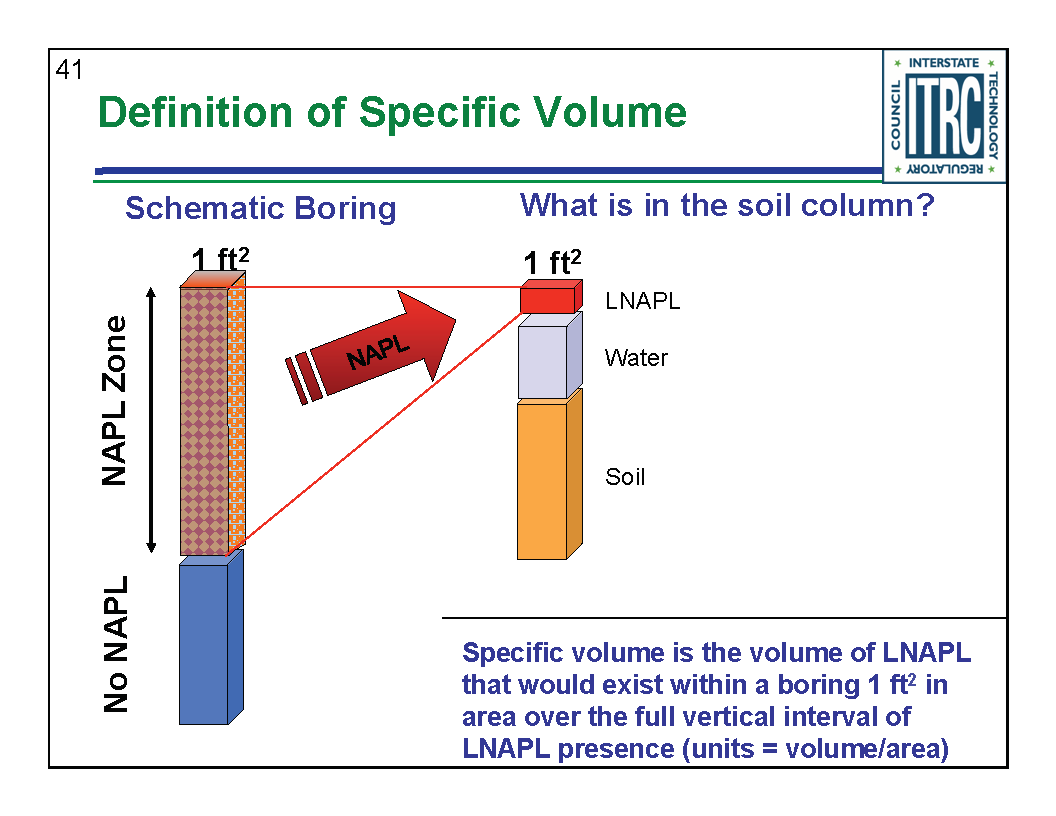
Introduction: Specific Volume
In the past, a common misconception of the vertical distribution of free product at the water table was based on the idea that LNAPL occurs as a distinct lens in which the drainable pore space is completely saturated with LNAPL and that the thickness of LNAPL in a monitoring well accurately represented the thickness of LNAPL in the formation. This was often referred to as the “pancake layer” model for LNAPL, but it does not reflect the important part soil properties play in the relationship between the amount of LNAPL in the formation and the thickness of LNAPL in a well (referred to as "apparent thickness").
In the table to the right, the amount of LNAPL in the formation for three different apparent LNAPL thicknesses in a monitoring well is described in terms of a “specific volume.” The specific volume is the volume of LNAPL in a given location divided by the surface area. This is a calculated value of the actual amount of LNAPL present in an area divided by the area. This would be the thickness of LNAPL that would remain in an LNAPL zone if the soil and water in that area were hypothetically removed.
For example, if there is one metre of LNAPL measured in a monitoring well screened in a sand, that corresponds to about 0.32 cubic metres (320 litres) of LNAPL per square metre of area. If this well was screened in a silt, there would only be about 0.040 cubic metres (40 litres) of LNAPL per square metre of area. This table shows the relationship between soil type, apparent LNAPL thickness, and the actual amount of LNAPL in the formation per square metre of area. The figure below shows how the ITRC
LNAPL Training Course describes LNAPL Specific Volume.
See the soil texture triangle to the bottom right to convert soil data in terms of % Sand, % Silt, and % Clay to the USDA soil classification system shown in the specific volume table to the right.
There are two types of specific volume:
Specific Volume: All the LNAPL present in the subsurface is used;
Mobile Specific Volume: Only the LNAPL present above the LNAPL residual saturation is used.
 Source: ITRC LNAPL Training
ITRC, 2014. “LNAPL Training Part 1: An Improved Understanding of LNAPL Behavior in the Subsurface".
| If a well has this much LNAPL: | |||
|---|---|---|---|
| 0.1 metre | 0.3 metre | 1 metre | |
| Soil Type | This much LNAPL is in the formation (m3/m2): | ||
| Silty Clay | 0.000041 | 0.00039 | 0.0045 |
| Silt | 0.00020 | 0.0028 | 0.040 |
| Loam | 0.00034 | 0.0058 | 0.084 |
| Sand | 0.0025 | 0.059 | 0.32 |
Table developed for Concawe Toolbox 2020 using LNAPL tool developed by
de Blanc, P. and S. K. Farhat, 2018. 25th IPEC: International Petroleum
Environmental Conference October 30 – November 1, 2018. Denver, Colorado.
Soil texture triangle showing the USDA classification system based on grain size and sand/silt/clay content (Public domain, Wikipedia)
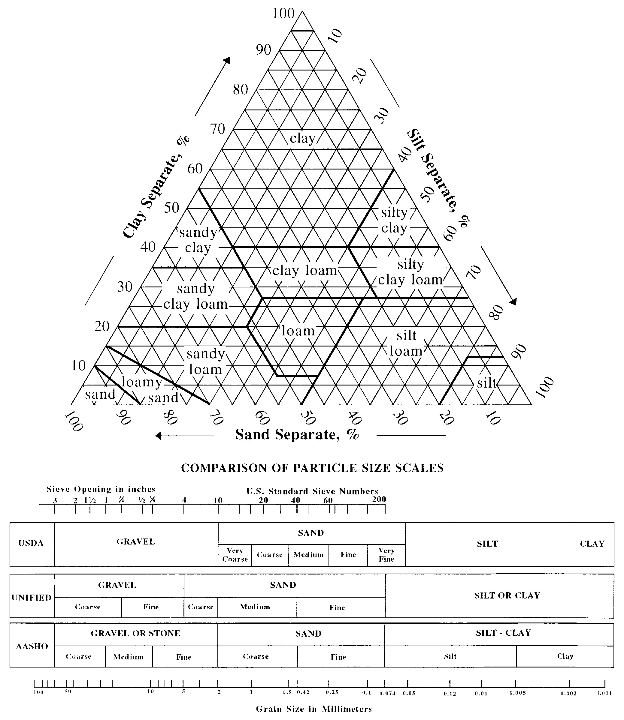
Learn more about soil classification systems
Multi-Site LNAPL Volume and Extent Model
What the Model Does
This tool calculates several key LNAPL values, including specific volume, recoverable volume, and transmissivity, at multiple locations for multiple layers of differing soil types. These values are used to calculate a total subsurface LNAPL volume. Based on LNAPL gradients specified by the user, estimated LNAPL velocities are also calculated. The distribution of calculated values is depicted graphically.
How the Model Works
The model is based on an extension of the methodology of the API’s LDRM (Charbeneau, 2007). The user enters data into three different input databases: 1) a soil parameter input database, 2) a well coordinate and fluid level gauging input database, and 3) a stratigraphy input database. The model determines the layers in which LNAPL is present, then calculates specific volume and other LNAPL parameters for the layered system. An area-weighted average of the specific volume is calculated to arrive at a total LNAPL volume.
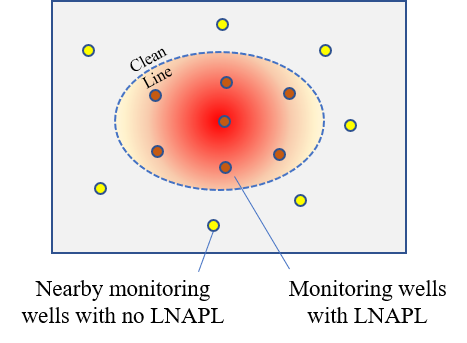
To improve the site-wide LNAPL volume calculations, it is important to include nearby monitoring wells that do not have any apparent LNAPL thickness in the monitoring well database. This will help establish a “clean line” around the LNAPL body and prevent extrapolation errors.
If you are just calculating the LNAPL volume in only a portion of an LNAPL body, use the polygon tool in the map to the right.
Input Data
Guidance on the selection of specific input parameters for this tool is provided in Section 4.2 of the User’s Manual which can be seen here:
More general guidance on parameters can be found in the API’s Parameter Selection Guide which can be downloaded here:
Key Assumptions
The model assumes that the LNAPL is in hydrostatic equilibrium with the surrounding media. Relative permeability is calculated by combining the Mualum model with the van Genuchten soil characteristic curve parameters (Charbeneau, 2007).
Developers
This LNAPL tool, sometimes referred to as the de Blanc LNAPL Model, was developed by Dr. Phil de Blanc and Dr. Shahla Farhat of GSI Environmental, Houston, Texas.
Charbeneau, 2007. LNAPL Distribution and Recovery Model (LDRM) Volume 1: Distribution and Recovery of Petroleum Hydrocarbon Liquids in Porous Media, Randall J. Charbeneau, American Petroleum Institute.
de Blanc, P.C. and S. K. Farhat, 2018. New Tool for Determining LNAPL Volume and Extent. GSI Environmental Inc. 25th International Petroleum Environmental Conference, October 30 – November 1, 2018, Denver, Colorado.
Inputs:
Will reset all input values.
Click Calculate to Update Maps and Model Output
Note: If extreme values are entered, model may crash and the website will have to be reloaded.
This is a relatively simple mapping system where a heat map is developed where a certain region around each well is assigned a color based on the parameter value for this well.
Control Parameters for Heat Map Appearance:
To refine the area of interpolation use the draw tools in the upper left-hand corner to draw the area you want to interpolate over. To remove the shape and reset the map click 'Calculate' again. At least 3 wells must be present for interpolation.
For more information, or to learn how to perform your own interpolation, go to this tutorial.
Information on this page can be downloaded using the button at the bottom of the page.
While the Concawe Toolbox includes the Tier 2 LNAPL Volume and Extent Model (de Blanc and Farhat, 2018) for evaluating how much LNAPL is present, another option is to apply the API LDRM Tool. These two tools can be found here:
- Multi-site LNAPL Model: Built into Concawe Toolbox Tier 2 under the questions “How much LNAPL is present?” and “Will LNAPL recovery be effective?”
- API LDRM: Download from the API web site here; requires Windows operating system. Note there are two separate manuals: Volume 1 provides background theory and conceptual models. Volume 2 is the actual User Guide with help on parameter selection.
Similarities Between Multi-site Model and LDRM
- Both calculate specific volume, recoverable volume, and transmissivity at individual well locations using the same relationships.
- Both use the f-factor method to calculate residual LNAPL saturation.
Differences Between Multi-site Model and LDRM
- LDRM has more choices for relative permeability calculation.
- LDRM allows users to account for smear zones above and below the LNAPL lens, while the Multi-site Model does not.
- LDRM allows users to specify a fixed or variable residual saturation or f-factor, while the Multi-site Model uses only a variable f-factor for residual saturation.
- LDRM simulates LNAPL recovery for several kinds of systems, while the Multi-site Model does not simulate LNAPL recovery.
- LDRM is limited to a 3-layer system, while the Multi-site Model considers up to 10 layers.
- LDRM is limited to a single location, while the Multi-site Model calculates LNAPL properties at unlimited locations simultaneously.
- The Multi-site Model estimates spatial variation of transmissivity and LNAPL volumes, while the LDRM does not.
- The Multi-site Model accesses a customizable soil properties database for different soil types, while the LDRM requires users to enter this information manually for every well.
Overview of LDRM
“The API LNAPL Distribution and Recovery Model (LDRM) simulates the performance of proven hydraulic technologies for recovering free-product petroleum liquid releases to groundwater. Model scenarios included in the LDRM are hydrocarbon liquid recovery using: single- and dual-pump well systems, skimmer wells, vacuum-enhanced well systems, and trenches. The LDRM provides information about LNAPL distribution in porous media and allows the user to estimate LNAPL recovery rates, volumes and times.” “The Guide has been designed to meet the needs of very busy professionals. As such, the primers and tools can be utilized within 15 to 25 minutes so that information can be gained rapidly. A list of references is also provided to enable more detailed understanding.” (API web page).
In general, the LDRM is a very powerful tool to simulate multiphase flow behavior that controls LNAPL recovery. To run LDRM, it is helpful to have an understanding of capillary pressure relationships (e.g., van Genuchten relationship; van Genuchten, 1980), LNAPL residual saturation concepts such as the f-factor, and the design of LNAPL recovery systems.
A short video describing LDRM can be viewed here.
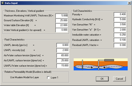
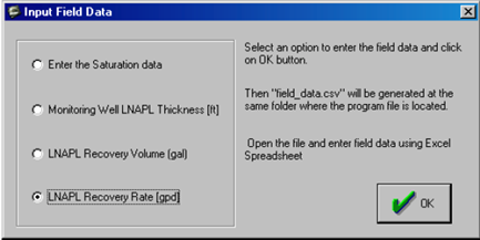
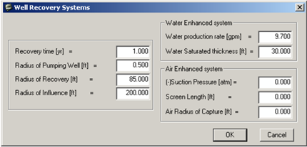
Checklist of Key LDRM Input Data
Images reproduced courtesy of the American Petroleum Institute from “LNAPL Distribution and Recovery Model (LDRM) Volume 2: User and Parameter Selection Guide”, API Publication 4760, January 2014
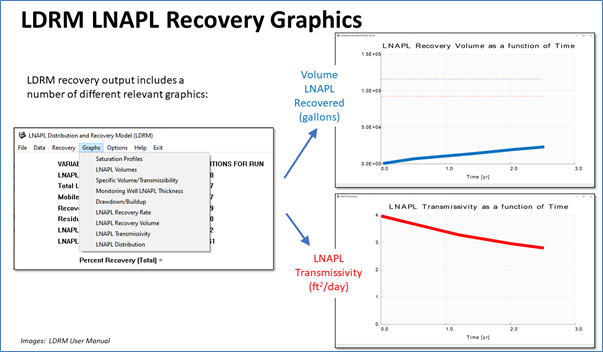
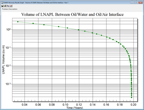
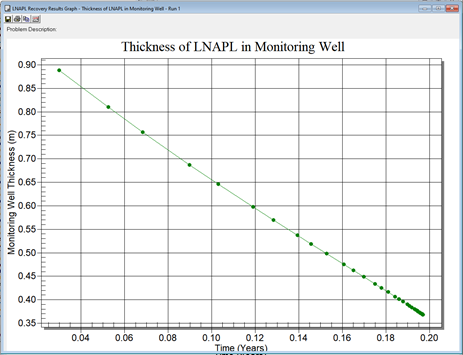
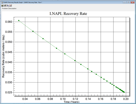
Example LDRM Output
Images reproduced courtesy of the American Petroleum Institute from LNAPL Distribution and Recovery Model, version 2.0, January 2007
Examples of the LNAPL recovery and LNAPL transmissivity graphics are shown below.
General LDRM Flowchart

LDRM Reference
Other References
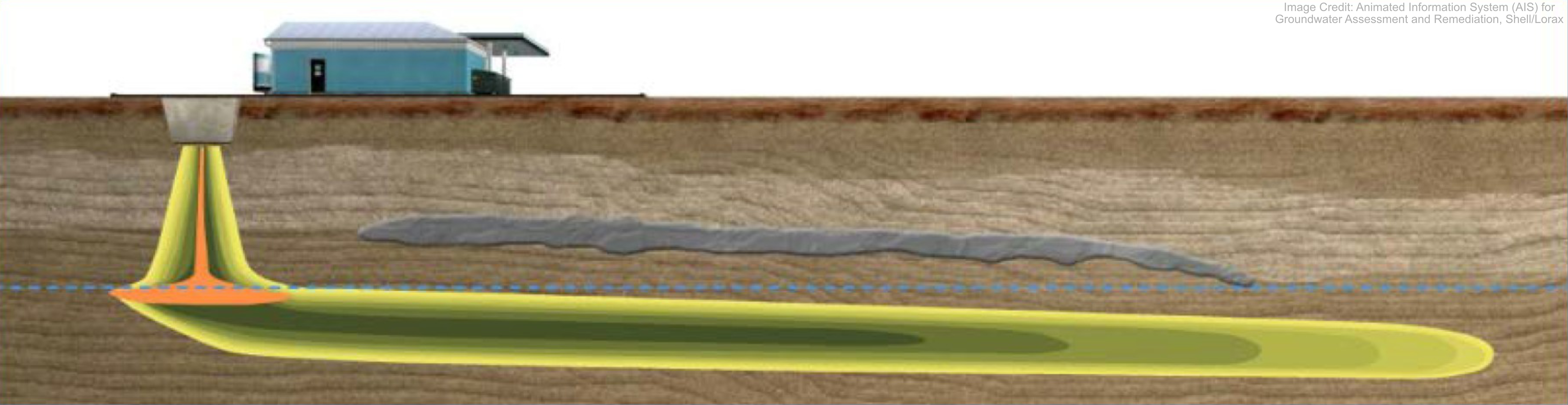
How far will the LNAPL migrate?
LNAPL Body Expansion and Eventual Stabilization Over Time
ITRC LNAPL Training Part 2: LNAPL Characterization and Recoverability – Improved Analysis, 2016.
The potential for LNAPL expansion is an important consideration when managing the risk from LNAPL at LNAPL sites. Some key conventions/concepts are:
- LNAPL experts typically call the LNAPL mass an “LNAPL Body” to prevent any confusion with a dissolved hydrocarbon plume that may be generated by the LNAPL. The phrase “LNAPL plume” should be avoided.
- LNAPL bodies need energy (pressure) to force the LNAPL at the leading edge of the LNAPL body into the pore space of the unimpacted soils.
- The required pressure can be significant, and once the release of LNAPL to the surface is stopped, the LNAPL body will stabilize at some point on its own accord because the pressure becomes insufficient to drive LNAPL into additional pore spaces.
- Recent advances in Natural Source Zone Depletion (NSZD) shows that NSZD is also an important process for limiting LNAPL migration and for stabilizing and even shrinking LNAPL bodies.
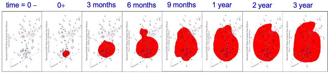
The figure above shows an example LNAPL body that was released at time 0 and then shows the size of the LNAPL footprint as indicated by monitoring wells over the next three years. The key point is that the footprint of most LNAPL bodies will stabilize after a few years after the release stops. Sale et al. (2018) describe this important point this way:
“A primary concern at LNAPL sites has been the potential for lateral expansion or translation of LNAPL bodies. Fortunately, long-term monitoring suggests that the extent of LNAPL bodies at older LNAPL releases tend to be stable, even when potentially mobile LNAPL exist within the LNAPL bodies (Mahler et al. 2012b). An important exception to stable LNAPL bodies is new releases. Historically, the primary explanation for the stability of older LNAPL releases has been low LNAPL saturation (fractions of pore space containing LNAPL) and correspondingly low formations conductivities to LNAPL. More recently, Mahler et al. (2012a) added the argument that natural loses of LNAPL play a critical role in controlling lateral expansion or translation of LNAPL bodies. In general, the threshold condition for expanding LNAPL bodies, at older release sites, is LNAPL release rates that are greater than natural source zone depletion rates. Much like dissolved phase petroleum hydrocarbon plumes, the extent of LNAPL bodies can be strongly limited by natural processes.”
LNAPL, 2014. “LNAPL Training Part 2: LNAPL Characterization and Recoverability – Improved Analysis”.
Mahler, N., Sale, T., Lyverse, M., 2012a. A mass balance approach to resolving LNAPL stability. Ground Water 50, 861-871.
Mahler, N., T. Sale, T. Smith, and M. Lyverse (2012b). Use of Single-Well Tracer Dilution Tests to Evaluate LNAPL Flux at Seven Field Sites, Journal of Ground Water, Vol. 50, No. 6, pp 851-860.
Sale, T., Hopkins, H., Kirkman, A., 2018. Managing Risk at LNAPL Sites. American Petroleum Institute, Washington, DC.
Kirkman LNAPL Body Additional Migration Tool
What the Model Does
This tool calculates the additional distance that the leading edge of an existing LNAPL plume is expected to migrate until it eventually stabilizes in the presence of natural source zone depletion (NSZD). To run the model you need to know three things about your LNAPL body: 1) a representative LNAPL transmissivity from bail down tests or from transmissivities calculated using the “LNAPL Volume Tier 2 Tool; 2) the measured LNAPL body gradient (the slope of the LNAPL body surface); and 3) the current LNAPL body radius (the model makes a simplifying assumption that the LNAPL body is circular).
How the Model Works
The model is based on multiple runs of the Hydrocarbon Spill Screening Model (HSSM; Weaver et al., 1994). For each run, an average LNAPL transmissivity (Tn) and gradient (i) were calculated across the oil lens at different times and for different soil types. These average properties were used as starting conditions to calculate the expected additional growth of an LNAPL body under one of five different NSZD rates using the steady-state relationship for a circular source derived by Mahler (Mahler et al., 2012)
The plot shows the calculated LNAPL body length increase for different average values of LNAPL transmissivity × gradient and piecewise linear fit to the data in the nomograph.
To use the model, enter the current LNAPL transmissivity (in m2/d) (see the bottom of the Tier 3 LNAPL Recovery tab), enter the LNAPL gradient (see Section 5.2.1.4 of the User Manual for a description), and select one of five different representative NSZD rates (see Tier 1 of the NSZD Estimation tab). The estimated additional LNAPL body growth from now will be automatically calculated. The model is a screening level model and will only give a general indication of the potential increase of the LNAPL body, but it will likely be more accurate than older models, such as HSSM, which do not account for NSZD processes.
Key Assumptions
The model assumes that there is an unlimited source of LNAPL and that the LNAPL flux is constant. This is an experimental model. Incorporation of HSSM (Weaver et al., 1994) and Mahler et al. (2012) represents a non-hysteric methodology where entrapment of LNAPL is ignored and loss rate inputs can account for partitioning and biodegradation losses.
Entrapment of LNAPL has been evaluated (Sookhak Lari et al., 2016; Pasha et al., 2014; Guarnaccia et al., 1997) and demonstrated to slow the rate of LNAPL migration. Current methods to incorporate entrapment require numerical models which are not within the scope of this tool. The lack of incorporating entrapment results in a conservative approach where the upper bound of LNAPL migration extent is estimated. The results of this tool are intended to be used for demonstrating LNAPL body stability by comparing the maximum potential for LNAPL migration to current extent.
The model is useful for estimating the upper bound of LNAPL migration. However, if the calculated LNAPL extent is used in cumulative LNAPL loss and time to depletion estimates then the resulting estimates would overestimate losses and underestimate time to depletion (Sookhak Lari et al., 2016). It is appropriate to use current delineated LNAPL body extent for cumulative loss calculations or time to depletion estimates.
Input Data
Guidance on the selection of specific input parameters for this tool is provided in Section 5.2.1 of the User’s Manual which can be seen here:
Developer
This LNAPL tool, referred to as the Kirkman LNAPL Body Additional Migration Tool, was developed by Andrew Kirkman of BP.
Guarnaccia, J. , Pinder, G. , Fishman, M. , 1997. NAPL: Simulator Documentation, US EPA.
Kirkman, A., 2021. LNAPL Body Additional Migration Tool. Andrew Kirkman, BP. Programmed by GSI Environmental.
Mahler et al., 2012. A mass balance approach to resolving LNAPL stability, N. Mahler, T. Sale, and M. Lyverse, Ground Water 50(6): 861-571, November/December 2012.
Pasha, A.Y. , Hu, L. , Meegoda, J.N. , 2014. Numerical simulation of a light nonaqueous phase liquid (LNAPL) movement in variably saturated soils with capillary hysteresis, Can. Geotech. J. 51, 1046–1062.
Sookhak Lari, K. , Davis, G.B. , Johnston, C.D. , 2016 Incorporating hysteresis in a multi-phase multi-component NAPL modelling framework; a multi-component LNAPL gasoline example, Advances in Water Resources. 96, 190-201.
Weaver et al., 1994. The Hydrocarbon Spill Screening Model (HSSM); Volume 1: User’s Guide, J.W. Weaver, R.J. Charbeneau, B.K. Lien, and J.B. Provost, U.S. EPA, EPA/600/R-94/039a.
Inputs:
Mahler LNAPL Migration Model
What the Model Does
Methods developed by Mahler et al. (2012) illustrate that natural losses of LNAPL (e.g., NSZD) can play an important role in governing the overall extent of LNAPL bodies. This module calculates the overall length of a contiguous LNAPL body, given an inflow of LNAPL rate, NSZD rate, and time period.
How the Model Works
The user is able to select a Long-Term LNAPL Release Rate, NSZD Rate, and a Time Period of Model. The output is an estimated ultimate LNAPL body length.
Key Assumptions
A limitation of the current methodology is the assumption of constant inflow of LNAPL throughout the entire lifetime of the LNAPL Body. Given either the reduction or termination of an LNAPL body, the times for stabilization and LNAPL body length could be much shorter. Additionally, LNAPL migration is not a function of the slope of the water table. Finally, the tool is limited to three different selections for the Long-term LNAPL Release Rate, three different selections for NSZD Rate, and three different selections for Time Period.
Input Data
Guidance on the selection of specific input parameters for this tool is provided in Section 5.2.2 of the User’s Manual which can be seen here:
Developer
This LNAPL tool was derived from the work of Mahler et al., 2012 by Poonam Kulkarni, GSI Environmental.
Kulkarni, P., 2021. LNAPL Migration Calculator based on Mahler et al. Model. Concawe LNAPL Toolbox.
Mahler, N., Sale, T., Lyverse, M., 2012. A Mass Balance Approach to Resolving LNAPL Stability. Groundwater 50, 861–871.
Inputs:
Information on this page can be downloaded using the button at the bottom of the page.
The Concawe Toolbox includes a new Tool developed by Andrew Kirkman based on LNAPL mass limitations included in the HSSM conceptual model integrated with LNAPL transmissivity relationships and LNAPL removal via Natural Source Zone Depletion (NSZD) using the Mahler et al. (2012) model. This Tier 3 section provides additional information about HSSM and UTCHEM, two tools that can be used to answer the question “How far will the LNAPL migrate?” The 2012 paper by Mahler et al. (2012) presents important findings on how NSZD limits LNAPL migration. Finally, an emerging LNAPL modeling method being developed by GSI’s Dr. Sorab Panday is a promising new approach where LNAPL modeling can be performed using a commonly used groundwater model like MODFLOW.
Overview of HSSM
- “HSSM” is an acronym for Hydrocarbon Spill Screening Model.
- Uses analytical relationships to simulate LNAPL movement.
- Simulates vertical LNAPL flow through the unsaturated zone.
- Simulates formation and decay of an LNAPL lens at the water table.
- Assumes a circular lens that is not affected by a water table slope.
- Simulates dissolution of LNAPL constituents and dissolved plume migration.
- Older model that requires workarounds to run on 64-bit operating systems like Windows 10.
- NSZD cannot be simulated, so that LNAPL spreading predictions in HSSM will overestimate actual spreading.
- Can be downloaded here.
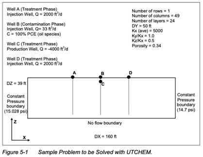
Overview of UTCHEM
- University of Texas chemical flood simulator developed for the oil industry.
- 3-D finite-difference numerical simulator for NAPL.
- Simulates multiphase, multicomponent, variable temperature systems and complex phase behavior.
- Accounts for chemical and physical transformations and heterogeneous porous media.
- Uses advanced concepts in high-order numerical accuracy and dispersion control and vector and parallel processing.
- Extremely powerful model but expensive and can be difficult to run.
- Due to its complexity, it is typically only used for more complicated LNAPL/environmental problems.
- Can be run either as a stand-alone program or accessed through GMS package (e.g., https://www.aquaveo.com/software/gms-groundwater-modeling-system-introduction)
Video
A short video describing HSSM and UTCHEM can be viewed here.
Overview of Mahler et al. (2012) LNAPL Stability Paper
- “...natural losses of light nonaqueous phase liquids (LNAPLs) through dissolution and evaporation can control the overall extent of LNAPL bodies and LNAPL fluxes observed within LNAPL bodies.”
- Uses proof-of-concept sand tank experiment where LNAPL is continually added but LNAPL body stabilizes due to losses via dissolution and evaporation.
- At actual LNAPL sites, LNAPL stability is rapidly achieved because of LNAPL losses via NSZD.
- Simple design charts are provided to show when LNAPL bodies will stabilize as a function of loading and NSZD rate, but these charts assume a constant LNAPL addition through time (a situation that is extremely infrequent at actual LNAPL sites).
- Key point: “...natural losses of LNAPL can play an important role in governing LNAPL fluxes within LNAPL bodies and the overall extent of LNAPL bodies.”
- The Concawe Toolbox Tier 2 model located under the question “How far will the LNAPL migrate?” developed by Andrew Kirkman uses key concepts from this paper to predict how far LNAPL can migrate.
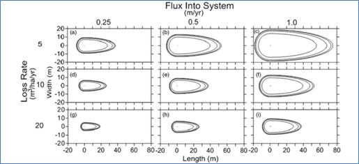
LNAPL body stabilization figure from Mahler et al. (2012). Each contour line is either 40 years (for panels a, b, c), 20 years (panels d, e, f), or 10 years (panels g, h, and i). (Reprinted with Permission)
Checklist of Input Data for HSSM
Appendix 3 of the HSSM User’s Guide (Weaver et al., 1994) lists key input data and provides support for parameter estimation. Key parameters with example values are reproduced below:
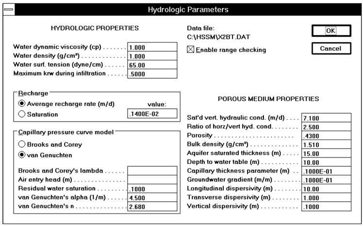
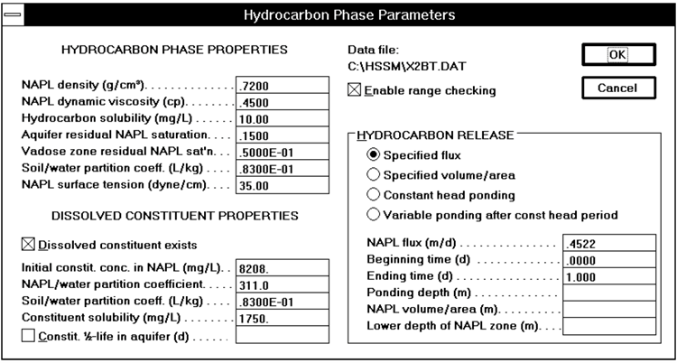
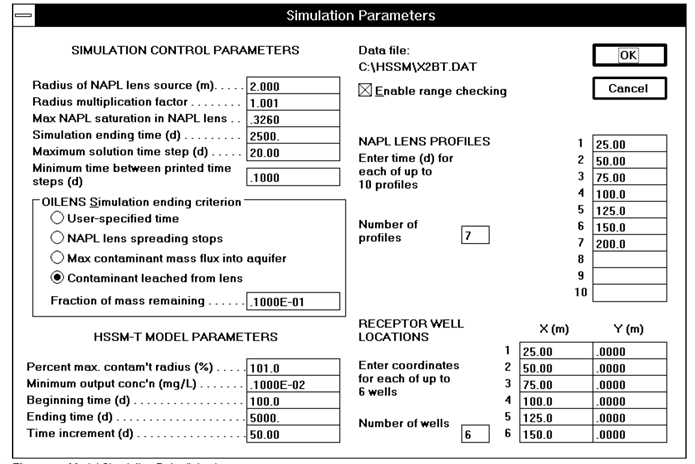
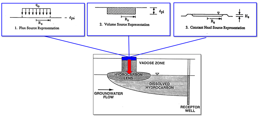
Users select one of three general release scenarios to the unsaturated zone and enter either an LNAPL flowrate over a certain time period, a volume of LNAPL released over a certain area, or a constant head of LNAPL in an impoundment.
General Flowchart for Running HSSM
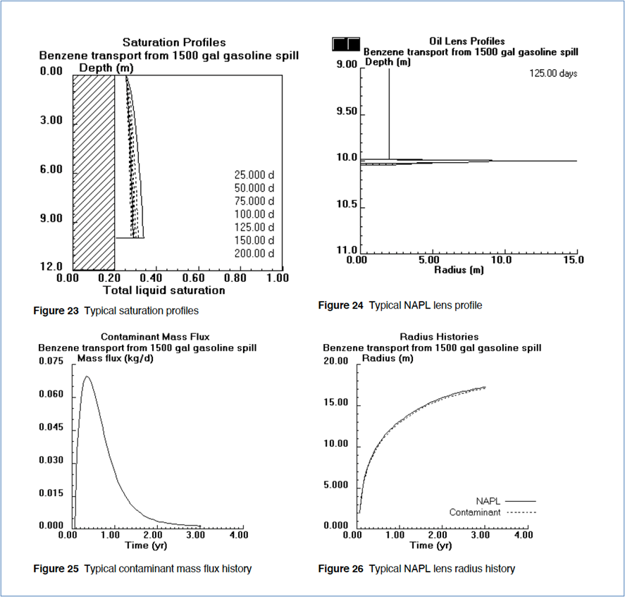
Example Output from HSSM
Example output is shown below (Weaver et al., 1994).
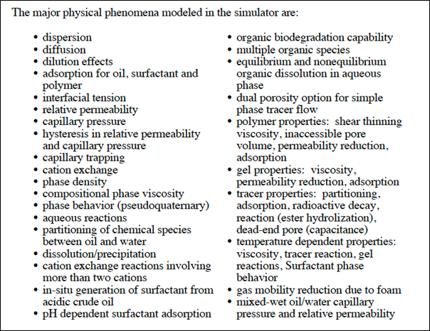
UTCHEM Key Processes that Require Input Data
The UTCHEM Users Guide provides this list of processes. For each process there are required input data. The overall list of potential input data is determined by the nature of the UTCHEM simulation.
Example UTCHEM Flowchart for a Surfactant Problem
An example problem in the GMS Tutorials Document (Aquaveo, 2021) outlines this process:
- Contamination: Define media and contaminant properties, initial and boundary conditions, and release.
- Dissolution: Equilibrium dissolution (only) from NAPL and conservative transport.
- Pre-flush PITT: A partitioning interwell tracer test (PITT) to assess NAPL saturations is simulated.
- Water Flush: A “pump and treat” simulation of 270 days of flushing using water. The results of this flush can be compared with the surfactant flush simulation.
- Surfactant Flush: A SEAR simulation using a surfactant to enhance dissolution and recovery with a 60-day simulation time.
- Post Flush: Simulation to determine recovery after the SEAR treatment is complete.
An Emerging LNAPL Model: The Panday LNAPL Simulator Based on MODFLOW
- Key Concept: Reduce governing multiphase flow equations using appropriate approximations to simplify and speed-up computations.
- Solve only one (LNAPL phase) equation for evaluating LNAPL flow in the vadose zone and along the water table.
- Assume air phase instantly equilibrates to movement of liquids.
- Valid for unsaturated zone flow (this is not a petroleum reservoir).
- Validated for flow of water in the vadose zone using Richards’ Equation.
- Eliminates air flow equation.
- Assume water saturation is unchanged by neglecting water flow dynamics and water redistribution.
- Appropriate at residual water saturations above capillary fringe.
- Neglects depression of water table by pressure of overlying LNAPL so that lateral LNAPL spread will be larger than computed so impact is conservative.
- Can bound impacts of LNAPL in capillary fringe and depression of water table.
- Eliminates water flow equation.
- Solve LNAPL flow equation only.
- Simplify constitutive relationships such that air-filled pore space is the porosity available for LNAPL flow—reduces 3-phase relations to standard 2-phase air-LNAPL equations readily solved by available unsaturated zone flow codes.
- Why is it important and useful?
- Can accommodate larger domain, finer grid, three-dimensional representation and structural complexity that may be difficult or impossible to represent and solve at a complex contaminated site with a multi-phase flow model.
- Significantly alleviates computational burden.
- Model runs quickly so that many alternative conceptualizations, parameter distributions, and ranges can be simulated to bracket likely behavior.
- Reduces parameterization burden (parameters are only needed for LNAPL phase).
- Parameterization of unsaturated and saturated zones at a site is difficult.
- Parameterization of multi-phase flow is difficult.
- Key Point: LNAPL migration can be performed with open source, public domain codes such as MODFLOW-USG or other unsaturated single phase flow codes.
- Current Status: A journal article is being prepared (Panday et al., in review) titled “Simulation of LNAPL flow in the vadose zone using a single-phase flow equation”. The abstract is reproduced below.
A simplified decoupled approach that considers flow only of the NAPL phase has been presented for simulating migration of LNAPL in the vadose zone and on the water table. The approach is applicable to several analyses of practical interest and can be readily adapted into existing vadose zone simulators by appropriate transformation of the constitutive relationships and parameters. Comparative examples demonstrate that results of LNAPL migration using the single-phase approach compare favorably to multiphase flow simulations in the vadose zone. The single-phase approach greatly reduces modeling effort and allows many more simulations to be performed within the same time period, than is possible with multiphase models. The main limitation of the single-phase approach is that it overestimates the spreading of LNAPL at the water table by about 10 to 20% in our comparative experiments for a flat water-table; these errors however reduce with increased water table gradients. The more rapid flow along the water table simulated by this approach as compared to the multiphase simulations is conservative for many examinations, however, this error is within the range of uncertainty in the impact of subsurface parameters such as intrinsic and relative permeability. If that is acceptable for an analysis, the single-phase approach presented here is a valid alternative for rapidly evaluating LNAPL migration in environmental settings.
References
Aquaveo, 2021. GMS Tutorials UTCHEM. Downloaded Feb. 2021.
EST, Aqui-Ver, 2006. API Interactive LNAPL Guide. American Petroleum Institute.
Panday, S., P. de Blanc, and R. Falta, in review. Simulation of LNAPL flow in the vadose zone using a single-phase flow equation. Submitted to Groundwater, in review (Feb. 2021).
University of Texas, 2000a. Volume I: User’s Guide for UTCHEM-9.0.
University of Texas, 2000b. Volume II: Technical Documentation for UTCHEM-9.0.
How long will the LNAPL persist?
Introduction
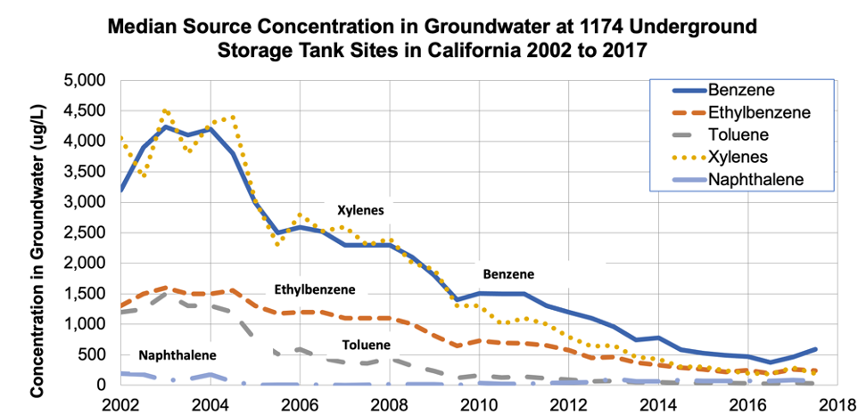
The figure to the right shows the median concentration in 1,174 Underground Storage Tank Sites in California over time. Because of stricter environmental regulations, the number and magnitude of releases has greatly diminished over time. In addition, almost all of these sites have had some form of source remediation, and all have benefitted from natural attenuation processes. Therefore, between 2004 and 2017, the median benzene concentration in groundwater at the highest concentration well in each of the 1,174 sites has been reduced by about 90%, from about 4,000 μg/L to about 500 μg/L (McHugh et al., 2013, 2019).
The table below shows the median change in benzene concentrations and in LNAPL apparent thickness from several hundred Underground Storage Tank Sites in California. Sites where companies were actively recovering LNAPL showed a benzene half-life (the time required for source zone monitoring well concentrations to decrease by 50%) of about 8 years, while sites with LNAPL in monitoring wells but no active remediation exhibited a benzene half-life of about 4 years. During the monitoring period, the thickness of the LNAPL in monitoring wells decreased by about 90% both for sites where active LNAPL recovery was on-going and sites where there was no active LNAPL recovery (Kulkarni et al., 2015).
Another resource is a simple nomograph method for screening estimates of LNAPL source mass depletion times, provided by Golder (2016). The nomographs can be used for estimating hydrocarbon mass depletion times resulting from biodegradation (mass loss rate) in the vadose zone and dissolution (mass loss rate) from the saturated zone.
Golder. 2016. “Toolkits for Evaluation of Monitored Natural Attenuation and Natural Source Depletion.” https://doi.org/Report Number: 1417511-001-R-Rev0. Contaminated Sites Approved Profession Society and Shell Global Solutions.
McHugh, T.E., Kulkarni, P.R., Newell, C.J., Connor, J.A., Garg, S., 2013. Progress in Remediation of Groundwater at Petroleum Sites in California. Groundwater 52, 898-907. (Updated by GSI Environmental, 2019).
Kulkarni, P.R., McHugh, T.E., Newell, C.J., Garg, S., 2015. Evaluation of Source-Zone Attenuation at LUFT Sites with Mobile LNAPL. Soil and Sediment Contamination: An International Journal 24, 917-929.
LNAPL Lifetime Model
What the Model Does
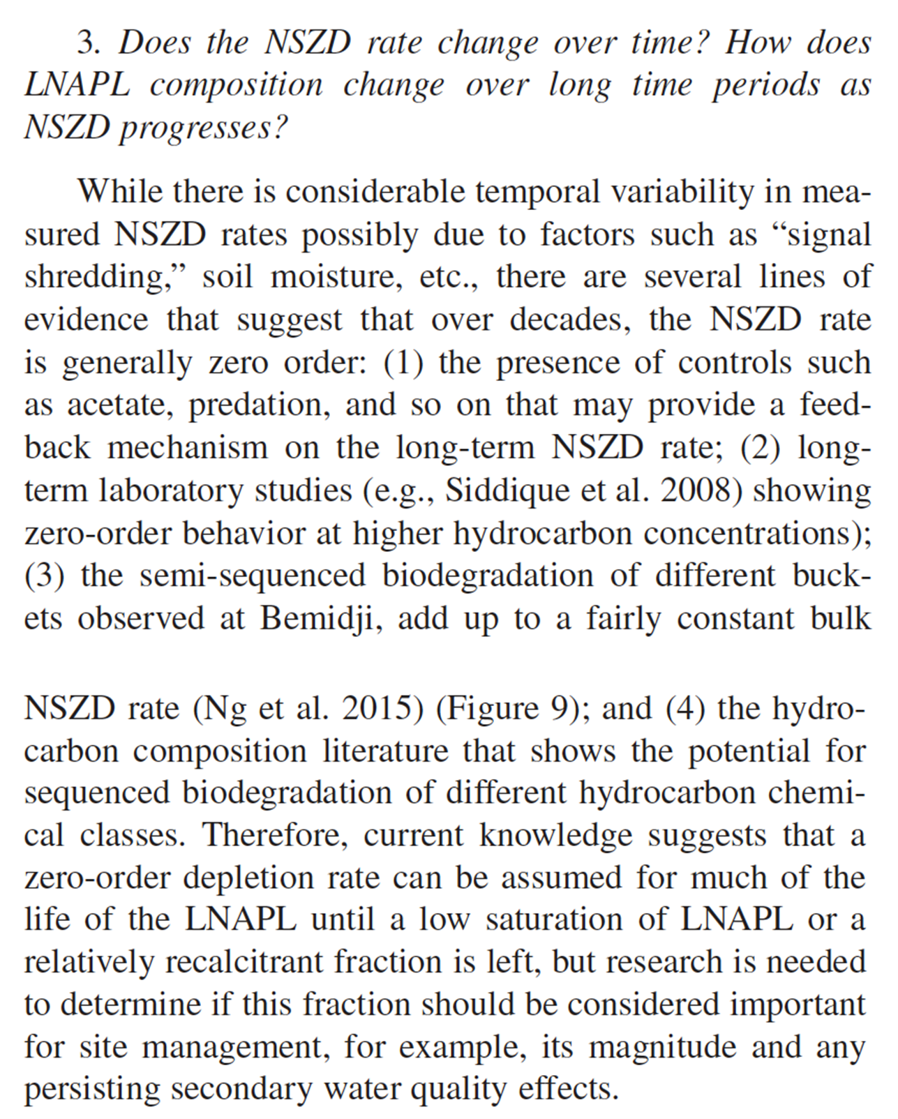
This simple LNAPL lifetime calculator shows two different models of how Natural Source Zone Depletion (NSZD) will remove LNAPL over time. * The left graph shows a “zero order” NSZD model where the current NSZD rate stays constant over a long period of time, as suggested by Garg et al. (2017) (see excerpt below). * The right graphs shows a “first order” NSZD model where the current NSZD rate drops in proportion to the mass of LNAPL remaining. Many natural attenuation models assume this type of relationship (e.g., BIOSCREEN model, Newell et al., 1996).
How the Model Works
Given an initial LNAPL body volume and NSZD rate (either via an NSZD study in the field or using typical NSZD rates in the scientific literature), the model calculates an estimated range when most/all of the LNAPL will be removed by NSZD. For example, one could take the estimated total LNAPL volume from the Tier 2 How Much LNAPL is Present? tool and enter this value as the Initial Volume of LNAPL Body in units of liters of LNAPL. The Model start year would be the year that the input data to the model were obtained.
Key Assumptions
The model assumes the user has an estimate of the LNAPL volume remaining in the subsurface (in volume units of total liters of LNAPL in the source zone) and has an estimate for the NSZD rates. Current knowledge suggests that a zero-order depletion rate can be assumed for much of the life of the LNAPL until a low saturation of LNAPL or a relatively recalcitrant fraction is left, but research is needed to determine if this fraction should be considered important for site management, for example, its magnitude and any persisting secondary water quality effects.
Overall, the linear model will present a best-case estimate for the LNAPL lifetime, and the first order model will be more conservative (i.e., may overestimate the LNAPL lifetime).
Input Data
Guidance on the selection of specific input parameters for this tool is provided in Section 6.2 of the User’s Manual which can be seen here:
NSZD values reported in the literature range from 2,800 to 72,000 liters per hectare per year with the middle 50% of NSZD values falling between 6,600 to 26,000 liters per hectare per year (Garg et al., 2017). More information is provided in “NSZD Estimation” under the Tier 3 tab.
Developer
This LNAPL tool was developed by Poonam Kulkarni of GSI Environmental.
References
Kulkarni, P., 2021. LNAPL Body Lifetime Calculator, Concawe LNAPL Toolbox.
Newell, C.J., D.T. Adamson, 2005. Planning-Level Source Decay Models to Evaluate Impact of Source Depletion on Remediation Timeframe. Remediation 15.
Newell, C.J., Gonzales, J., McLeod, R. , 1996. BIOSCREEN Natural Attenuation Decision Support System. U.S. Environmental Protection Agency. (https://www.gsi-net.com/en/software/free-software/bioscreen.html)
Garg, S., C. Newell, P. Kulkarni, D. King, M. Irianni Renno, and T. Sale, 2017. Overview of Natural Source Zone Depletion: Processes, Controlling Factors, and Composition Change. Groundwater Monitoring and Remediation 37. (open access; https://ngwa.onlinelibrary.wiley.com/doi/full/10.1111/gwmr.12219).
Inputs:
LNAPL Body Lifetime assuming constant NSZD rate over time.
LNAPL Body Lifetime assuming NSZD rate decreases proportional to the LNAPL mass remaining.
Information on this page can be downloaded using the button at the bottom of the page.
A simple box model is provided in Tier 2 and provides a range of time required for the LNAPL to be removed by Natural Source Zone Depletion (NSZD). Users enter the estimated mass/volume of LNAPL present and the estimated NSZD rate.
Two more sophisticated computer tools that can be used to estimate how long the LNAPL might persist at a site are REMFuel (Falta et al., 2012) and LNAST (Huntley and Beckett, 2002). A short summary of each model is provided below:
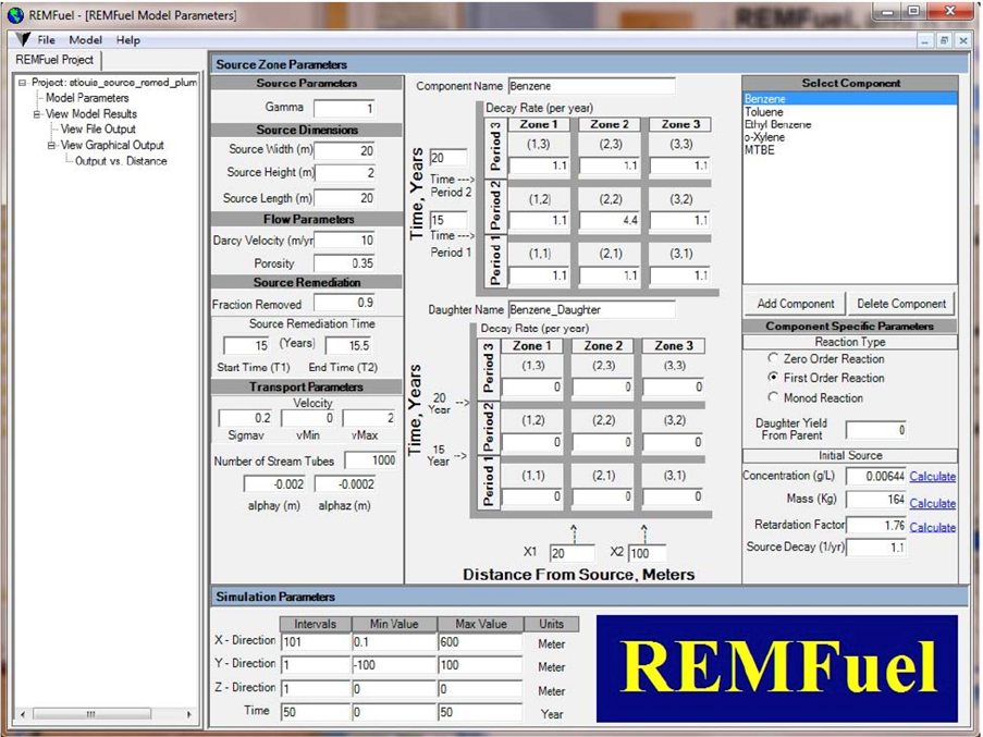
Overview of REMFuel
- REMFuel is a coupled analytical source zone/plume response model distributed by USEPA.
- Based on popular REMChlor model used at chlorinated solvent sites.
- The source zone model includes a box model where the mass of the dissolution product to be modeled is entered and a relationship “gamma” that describes the mass flux out of the source at any time compared to the remaining mass is specified by the user.
- Solute transport model simulates advection, dispersion, retardation, sorption assuming simple 1-D groundwater flow.
- The user can specify any percent of source removal at any time to model plume response to active remediation.
- The user can model plume remediation at any time in three separate spatial zones by increasing first order decay constants.
- NSZD can also be simulated by entering a value for “Source Decay” although there is no discussion in User’s Guide on how to do this.
- Key output of the model are graphs showing the concentration (or mass discharge) of the constituents in the dissolved plume vs. distance from source.
- Download model from USEPA web page here.
Overview of API’s LNAPL Dissolution and Transport Screening Tool (LNAST; version 2.0.4)
- LNAST is suite of calculation tools, information about LNAPL, and LNAPL parameter databases. LNAST focuses on LNAPL distribution and fate at the water table. The calculation tool part of LNAST:
- Predicts LNAPL distribution, dissolution, and volatilization over time.
- Calculates downgradient dissolved-phase concentration through time.
- Shows results both with and without hydraulic recovery of LNAPL.
- LNAST simulates the smear zone and the downgradient dissolved plume.
- Combines multi-phase transport, dissolution, and solute transport.
- Accounts for relative permeability effects caused by LNAPL.
- Zones of high LNAPL saturation have much less groundwater flow through them, extending the longevity of these zones.
- Good tool for estimating how long an LNAPL-generated plume will persist.
- Powerful tool to see if LNAPL recovery reduces the longevity of the source and plume.
- Key output is concentration of dissolved constituents in the plume vs. time at an observation well.
- Does not account for NSZD.
- Assumes that remediation occurs shortly after the LNAPL release. You cannot release LNAPL many years ago and then start the remediation now a few decades later.
- LNAST can be downloaded here.
Videos
Two short videos are available to learn more about REMFuel and LNAST:
Checklist for REMFuel Input Data
Key input data are shown below. One key feature is that the plume produced by the source can be broken up into nine “space-time” domains with three separate time periods and three separate spatial zones. For example, the first third of the plume downgradient from a 40-year-old source can have its own first order decay coefficients for three separate time periods, such as a 20-year natural attenuation period, then a 5-year plume remediation period, then a 15-year post-remediation natural attenuation period.
While much of the input data below is commonly collected during site characterization activities (e.g., Darcy groundwater velocity, source width/height/length, porosity) the source zone gamma term may be unfamiliar to many users. Basically, gamma defines the relationship between mass flux leaving the source and the remaining mass in the source at any time. For example:
- Gamma of zero results in a constant source mass flux until mass is gone, then zero flux (a step function).
- Gamma of 0.5 results in a linear decline in source concentration based on the amount of LNAPL mass originally released and the original source concentrations.
- Gamma of 1.0 results in an exponential decline in source concentration based on the amount of LNAPL mass originally released and the original source concentrations (this is often used as a default value).
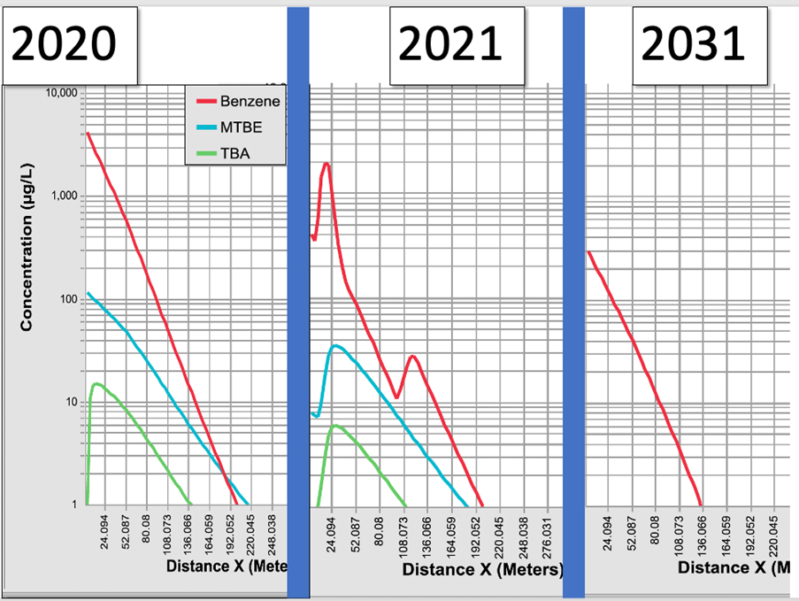
Example of REMFuel Output Data for Three Separate Time Periods
In this example, source remediation and plume remediation were performed, leading to the spikey concentration vs. distance curves in the 2021 panel (see the REMFuel video for a more detailed explanation). Note that the Y-axis is log-scale.
Checklist of Input Data for LNAST
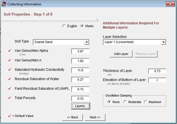
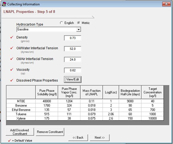
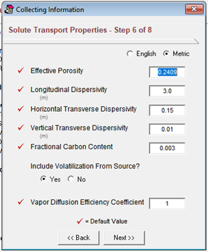
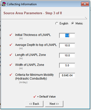
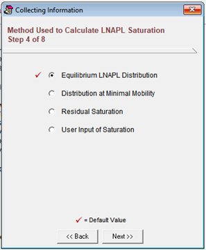
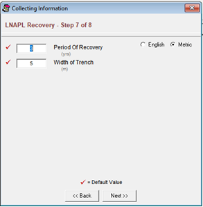
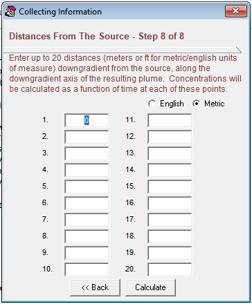
Images reproduced courtesy of the American Petroleum Institute from LNAPL Dissolution and Transport Screening Tool, version 2.0.4, February 2006To use LNAST, the user first indicates the information desired from the tool:
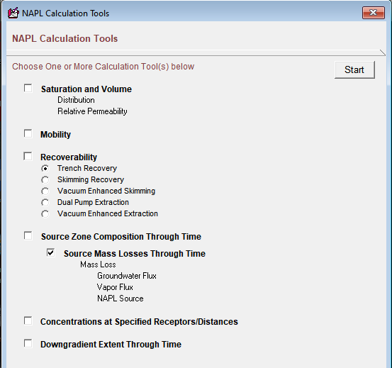
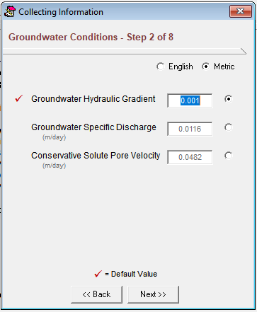
The tool then takes the user through a series of eight input screens to define soil properties, groundwater conditions, source area parameters, LNAPL properties, and solute transport.


Example of LNAST Output Data
Images reproduced courtesy of the American Petroleum Institute from LNAPL Dissolution and Transport Screening Tool, version 2.0.4, February 2006
After performing the selected calculations, LNAST allows users to display results to the screen, create a report, or export the results.
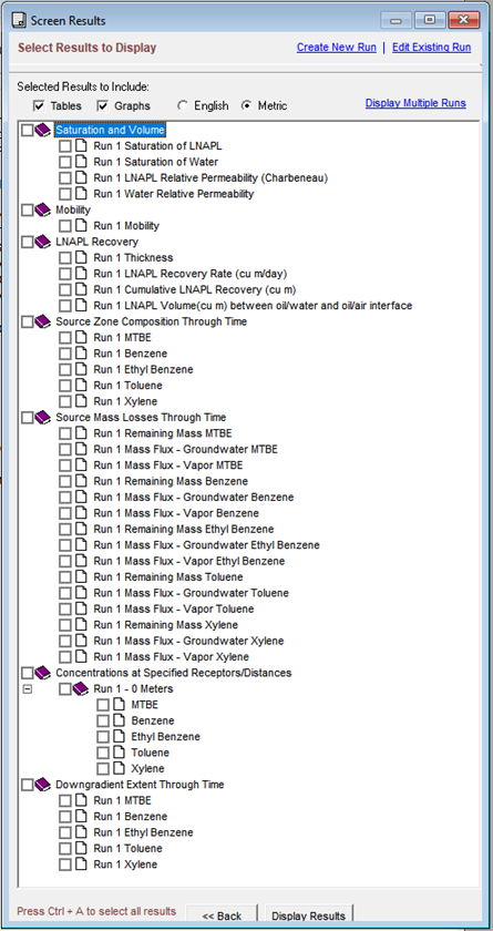
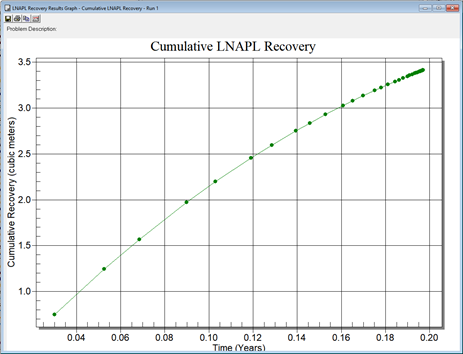
An example of key output for LNAPL recovery in a trench is shown below:


References
How will LNAPL risk change over time?
Introduction
The potential risk associated with LNAPL composition can change over time as the LNAPL is weathered due to Natural Source Zone Depletion (NSZD), often decreasing over time. This reduction in risk over time increases the reliability of NSZD as a long-term LNAPL management strategy. The table below shows an approximate way to conceptualize the change in risk as LNAPLs weather. At most LNAPL sites, most of the risk in groundwater exposure pathways are associated with the amount of benzene that is present in the LNAPL. The higher the mole fraction of benzene in the LNAPL, the higher the potential concentration of dissolved benzene in groundwater. In this example, the composition of a fresh gasoline and a weathered gasoline were taken from a 1990 paper by Johnson et al. As can be seen in the table, the fresh gasoline had a benzene mole fraction of 0.0093 (calculated from a mass fraction of 0.0076 or about 1% by weight) (column 2). These calculations assumed a temperature of 20°C and 1 atmosphere pressure. The weathering process removes benzene, and the weathered gasoline mole fraction was 0.0028 (mass fraction of 0.0021) (column 3). When the mole fractions are multiplied by a pure-phase effective solubility (column 4), a theoretical concentration in groundwater can be calculated for water in perfect equilibrium with the LNAPL (columns 5 and 6). Then, using common regulatory criteria in the U.S. for allowable concentrations in drinking water (column 7), a relative risk (RR) factor was calculated for both the fresh and weathered gasoline (columns 8 and 9) where the equilibrium water concentration is divided by the regulatory criteria. As shown in columns 8 and 9, benzene by far has the highest regulatory risk.
The bottom right of the table shows the cumulative relative risk for the BTEX compounds and naphthalene was 3,285 for the fresh gasoline but only 1,020 for the weathered gasoline. Therefore, in this simple example, the relative risk associated with the LNAPL was reduced by almost 70% when going from a fresh gasoline to the weathered gasoline sample. This is only an example of how the hypothetical risk of LNAPL can change over time due to LNAPL attenuation processes over time. Although each site will be different, in general LNAPL attenuation processes will reduce the risk associated with groundwater exposure pathways over time.
Johnson, P.C., M.W. Kemblowski, and J.D. Colthart. 1990. Quantitative Analysis of Cleanup of Hydrocarbon-Contaminated Soils by In-Situ Soil Venting. Ground Water, Vol. 28, No. 3. May – June 1990, pp 413-429.
Newell, C.J.. and T. McHugh, 2021. LNAPL Risk Change Over Time Example, Concawe LNAPL Toolbox.
Entire LNAPL Composition (Mass Fraction) Dataset from Johnson et al. (1990) Used in Hypothetical Example Above
LNAPL Dissolution to Groundwater Model
What the Model Does
This model calculates the theoretical concentration of dissolved hydrocarbons in groundwater downgradient of an LNAPL source over time due to dissolution processes. The model produces a graph of dissolved constituent (such as B,T,E, X and MTBE) in groundwater over time in units of mg/L as an LNAPL source is depleted of these soluble constituents.
How the Model Works
A known volume of LNAPL is released to the subsurface. The LNAPL is comprised of several components whose volume fractions and densities are known. The unidentified fraction of the LNAPL is a mixed petroleum product with unknown components, but with a known average molecular weight and density.
The LNAPL establishes a lens in the groundwater with a known width and average thickness. Groundwater flows through the LNAPL lens and dissolves the LNAPL constituents, reducing the remaining volume of LNAPL and changing its composition as the more soluble compounds dissolve out of the LNAPL. Equilibrium between the water and LNAPL within the lens is assumed, so that the concentration of constituents downgradient of the LNAPL are equal to the effective solubility of the LNAPL constituents. Effective solubility is the solubility of a pure phase component times its mole fraction in the LNAPL.
The key strengths of the model are:
- The model is simple and easy to understand.
- Because of its simplicity, the model can be modified by users if needed.
Weakness of the model are:
- Equilibrium is unlikely to be completely achieved at actual sites, so the model over-estimates downgradient aqueous phase concentrations.
- The explicit solution scheme can become inaccurate or unstable if the time step is too large.
Key Assumptions
Key assumptions of the model are as follows:
- The groundwater concentration is directly downgradient of the LNAPL body before any attenuation or mixing occurs.
- Volume is conserved upon fluid mixing.
- The concentration of a constituent in the aqueous phase in equilibrium with the LNAPL is the constituent’s mole fraction in the LNAPL times the constituent’s pure phase solubility.
- Water exiting the LNAPL lens is saturated with each LNAPL constituent; i.e., there is perfect mixing between groundwater and LNAPL constituents in the LNAPL lens.
- LNAPL does not impede groundwater flow.
- Fluid densities and solubilities do not change significantly with temperature.
- The change in total number of moles in the LNAPL is slow over the time period of the model.
Input Data
Many laboratory analysis of LNAPL show composition as mass concentrations (mg/L). To convert a mass concentration of a constituent like benzene to a volume fraction, you will need to divide the mg/L value by the density of the constituent (78,000 mg per gram-mole for benzene). So 1 mg/L benzene concentration in LNAPL becomes a volume fraction of 1.3x10⁻⁵ Liters benzene per Liter of LNAPL (unitless).
Guidance on the selection of specific input parameters for this tool is provided in Section 7.2 of the User’s Manual which can be seen here:
Developer
This LNAPL tool was developed by Dr. Phil de Blanc, GSI Environmental.
de Blanc, P., 2021. LNAPL Dissolution Calculator, Concawe LNAPL Toolbox.
Model Inputs:
Click Calculate to Update Plot
Note: If the calculated solution appears to be unstable try reducing the model time step.
LNAPL Constituents Chemistry Inputs:
Add up to 5 constituents. Double click to editInformation on this page can be downloaded using the button at the bottom of the page.
The risk posed by the toxic components of an LNAPL plume is a function of the constituents’ concentration in groundwater in contact with the LNAPL. A multi-component LNAPL dissolution model based on the LNAPL constituent mole fraction and Raoult’s law (Mayer and Hassanizadeh, 2005) is provided in Tier 2 and shows how the dissolved constituent concentrations immediately downgradient of an LNAPL body change over time.
A more sophisticated computer tool, API’s LNAST model, also shows the change in dissolved phase LNAPL concentrations over time (Huntley and Beckett, 2002). It is summarized below. Finally, two other key LNAPL attenuation studies, a LNAPL mass balance developed by Ng et al. (2014) and a 2003 report about weathering of jet fuel LNAPL, are also reviewed below.
Overview of API’s LNAPL Dissolution and Transport Screening Tool (LNAST)
- LNAST is suite of calculation tools, information about LNAPL, and LNAPL parameter databases. LNAST focuses on LNAPL distribution and fate at the water table. The calculation tool part of LNAST:
- Predicts LNAPL distribution, dissolution, and volatilization over time.
- Calculates downgradient dissolved-phase concentration through time.
- Shows results both with and without hydraulic recovery of LNAPL.
- Simulates the smear zone and the downgradient dissolved plume.
- Combines multi-phase transport, dissolution, and solute transport.
- Accounts for relative permeability effects caused by LNAPL.
- Zones of high LNAPL saturation have much less groundwater flow through them, extending the longevity of these zones.
- Good tool for estimating how long an LNAPL-generated plume will persist.
- Powerful tool to see if LNAPL recovery reduces the longevity of the source and plume.
- Key output is concentration of dissolved constituents in the plume vs. time at an observation well.
- Does not account for Natural Source Zone Depletion (NSZD).
- Assumes that remediation occurs shortly after the LNAPL release. You cannot release LNAPL many years ago and then start the remediation now a few decades later. The REMFuel model will do this, see Tier 3 of “How long will LNAPL persist?” portion of the Concawe LNAPL Toolbox.
- LNAST can be downloaded here.
Video
A short video to learn more about LNAST can be found here.
Checklist of Input Data for LNAST
Images reproduced courtesy of the American Petroleum Institute from LNAPL Dissolution and Transport Screening Tool, version 2.0.4, February 2006
To use LNAST, the user first indicates the information desired from the tool:

The tool then takes the user through a series of eight input screens to define soil properties, groundwater conditions, source area parameters, LNAPL properties, and solute transport.


Example of LNAST Output Data
Images reproduced courtesy of the American Petroleum Institute from LNAPL Dissolution and Transport Screening Tool, version 2.0.4, February 2006
After performing the selected calculations, LNAST allows users to display results to the screen, create a report, or export the results.

An example of key output for LNAPL recovery in a trench is shown below:

Description of Ng et al. (2014) LNAPL Model
- A reactive transport model of an LNAPL body was developed by Ng et al. to simulate a 1979 LNAPL release at what is now the National Crude Oil Spill Research Site.
- The model was based on extensive research conducted by the USGS and several universities to construct the model.
- As shown in the figure below developed by Garg et al. (2017), Ng et al. developed a mass balance around five “buckets”: BEX, toluene, short-chained alkanes, long-chained alkanes, and pre-NVDOC (non-volatile dissolved organic carbon).
- The figure shows the percent depleted of each bucket in 27 years (green values), the contribution to the NSZD rate (red values), the rate of biodegradation of each bucket (blue arrows), and an inhibition term (red arrows).
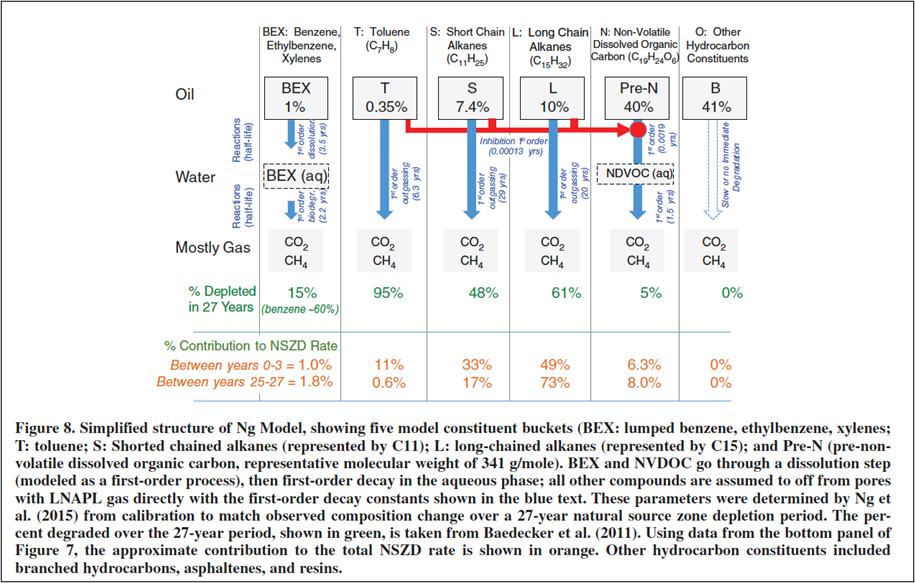
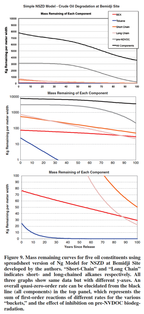
- The Ng et al. model was used to simulate LNAPL composition from the 1979 to the year 2079 as shown to the right (Garg et al. 2017).
- It assumed the “overall NSZD rate is approximately constant over time (pseudo-zero order), because the main contributors to NSZD, the short-chained and long-chained alkanes, are represented as a first-order decay rate where the biodegradation rate for these two constituent ‘buckets’ gets smaller over time. As they do, the inhibition effect on the pre-NVDOC bucket defined by Ng et al. (2014, 2015) diminishes and the pre-NVDOC starts to biodegrade and ‘take up the slack’ for the declining alkane degradation rate to produce a relatively constant biodegradation rate for much of the site history.” (Garg et al. 2017).
- Overall, “the detailed reactive transport model developed by Ng et al. (2014, 2015) was adapted to explore LNAPL composition change as a result of NSZD. This model suggests that methanogenic microorganisms consume different LNAPL constituents/chemical classes in a semi-sequential basis due to inhibition and other effects, which then can produce quasizero- order bulk NSZD rates over long time periods” (Garg et al. 2017).
Parsons Fuel LNAPL Weathering Study
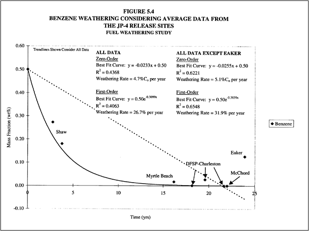
- Study of 12 LNAPL sites where data on concentration of BTEX constituents in LNAPL (as weight percent) vs. time (over the span of several years) in LNAPL source zones was compiled (Parsons et al., 2003). Jet fuel (JP-4) was the LNAPL found at most of these sites.
- “Free-phase fuel BTEX weathering rates will vary from site to site and are influenced by many factors including spill age, the relative solubility of individual compounds, free product geometry, and the rate at which groundwater and precipitation contacts LNAPL.”
- “…the average total BTEX, first-order weathering rate for five JP-4 sites is approximately 16 %/yr. Based on all of the data collected, this appears to be a reasonable default value for estimating total BTEX weathering from JP-4 LNAPL.”
- “As predicted by their relatively high solubilities, benzene and toluene exhibit higher weathering rates than ethylbenzene and xylenes. Because benzene is a known human carcinogen with a federal MCL of 5 μg/L, benzene weathering rates will generally determine the timeframe for fuel spill remediation.” “Based on Figure 5.4, the average benzene first-order weathering rate for five JP-4 sites is approximately 26 %/yr. Based on all of the data collected, this appears to be a reasonable default value for estimating benzene weathering from JP 4 LNAPL.”
References
Will LNAPL recovery be effective?
Introduction
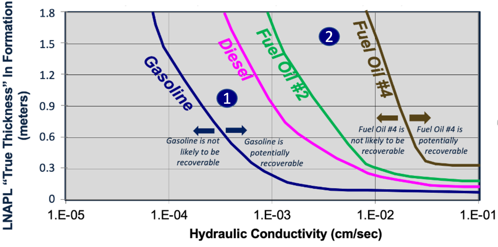
The Texas Risk Reduction Program developed guidance for managing LNAPL in the subsurface and provided a quantitative screening tool for knowing when LNAPL is potentially recoverable using total fluids submersible pumps. This tool was developed by entering certain site conditions into the numerical multiphase transport model ARMOS. Key assumptions included: petroleum hydrocarbon contamination and a single submersible total-fluids recovery pump with an inlet set at depth of 3 feet (1 metre) below static water level. The figure to the right summarizes the results of numerous model simulations configured for different fuel viscosities, hydraulic conductivities, product thicknesses, and recovery system drawdown that are combined with assumptions of what constitutes recovery effectiveness at this site.
This tool provides an approximate indicator of recoverability based on the new LNAPL paradigm that soil type and the LNAPL vertical equilibrium model are key recoverability factors. The Texas Risk Reduction Program described this curve as an example quantitative screen for conventional NAPL recovery and recommended it not be used on a site-specific basis. However, several members of the original TRRP guidance did feel it could provide a rapid planning level method to evaluate recoverability, and therefore this tool is used as a Tier 1 tool for the Concawe toolbox. For a more detailed evaluation of recoverability, use the Multi-Site LNAPL Volume and Extent Model (How Much LNAPL is Present, Tier 2) or use the LNAPL transmissivity calculator (Will LNAPL recovery be effective, Tier 2).
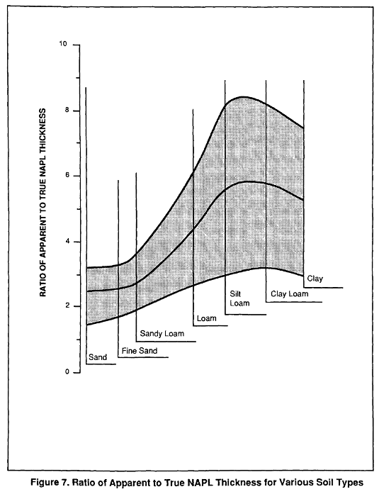
Step 1
Get the Ratio of Apparent Thickness to “True Thickness” (now referred to as “specific volume”) based on soil type (Reidy et al., 1990).
Step 2
Multiply this Ratio by the apparent thickness (measured thickness) in the monitoring well of interest to get a soil type adjusted estimate for True Thickness (“specific volume”).
Step 3
Use the calculated True LNAPL Thickness in Step 2 on the Y-axis of the chart below.
Step 4
Use the hydraulic conductivity of the formation at the monitoring well of interest on the X-axis of the chart below.
Step 5
Mark a point on the graph where the values for the Y-axis and X-axis intersect (see Example 1 dot for gasoline and Example 2 dot for Fuel Oil #4).
Quantitative Screening Tool for Determining if LNAPL Recovery is Feasible Using LNAPL Pumping
Step 6
If the intersection of the two values for the X- and Y-axes are to the right of the line for your LNAPL type, it suggests that LNAPL is potentially recoverable (see Example 1 for gasoline below, this point is to the right of the gasoline line and therefore may be recoverable).
If the intersection of the two values for the X- and Y-axes are to the left of the line for your LNAPL type, it suggests that LNAPL is likely not recoverable (see Example 2 for Fuel Oil #4 below, this point is to the left of the Fuel Oil #4 line and therefore is less likely to be recoverable).
Texas Risk Reduction Program, 2013. Risk-Based NAPL Management, TRRP-32. Austin, Texas.
Reidy, P.J., Lyman, W.J., Noon, D.C., 1990. Assessing UST Corrective Action Technologies. Early Screening of Clean-up Technologies for the Saturated Zone. U.S. EPA, EPA/600/2-90/027.
LNAPL Transmissivity Calculator
What the Model Does
This tool calculates the following variables that indicate LNAPL volume and mobility at a single location for a single soil type: LNAPL specific volume, transmissivity, and Darcy flux. LNAPL transmissivity is the product of the average LNAPL hydraulic conductivity times the thickness of the LNAPL lens. Large transmissivity values indicate that LNAPL has greater potential to move through the subsurface than small values and suggests that LNAPL may be more easily mobilized or recovered. Transmissivity is often used as an indication of when LNAPL recovery is no longer practical.
How the Model Works
The model is based on the methodology of the API’s LDRM (Charbeneau, 2007). The user enters parameters for the soil type, fluid properties, and the thickness of LNAPL observed in a monitoring well. LNAPL saturations are computed over the LNAPL thickness to calculate specific volume. Transmissivity is then calculated by integrating the saturation-dependent relative permeability over the LNAPL thickness. The product of the average relative permeability and the saturated hydraulic conductivity for the LNAPL is the LNAPL transmissivity. The transmissivity divided by the LNAPL thickness, then multiplied by the LNAPL gradient (see Section 5.2.1.4 of the User Manual for a description) is the LNAPL Darcy flux (volume of LNAPL per unit area of formation). The model uses an “f-factor” approach in which the LNAPL residual saturation is a function of the LNAPL thickness across the lens (Charbeneau, 2007).
Based on guidance from ITRC (2018) the key threshold for LNAPL recovery is the LNAPL transmissivity has to be higher than this general range of numbers: 0.0093 to 0.074 m2/day . If the calculated or measured LNAPL transmissivity is below that the lowest value, then there is a high probability that LNAPL hydraulic recovery will not to be cost effective or efficient. If above the highest number, then hydraulic recovery has a much higher likelihood of being feasible. Wells exhibiting LNAPL transmissivity values within this range are likely dominated by residual LNAPL. These values account for multiple soil and LNAPL types (ITRC, 2018).
Key Assumptions
The model assumes that the LNAPL is in hydrostatic equilibrium with the surrounding media. Relative permeability is calculated by combining the Mualum model with the van Genuchten soil characteristic curve parameters (Charbeneau, 2007).
The model uses default values for various soil and LNAPL properties. Soil properties can be found in Carsel and Parrish (1988), and LNAPL properties can be found in Mercer and Cohen (1990) and Charbeneau (2003).
Input Data
Guidance on the selection of specific input parameters for this tool is provided in Section 8.2.3 of the User’s Manual which can be seen here:Developer
This LNAPL tool was developed by Dr. Phil de Blanc, GSI Environmental.
Carsel, R.F., and R.S. Parrish. 1988. Developing joint probability distributions of soil water retention characteristics. Water Resour. Res. 24:755-769.
Charbeneau, R. 2003. Models for Design of Free-Product Recovery Systems for Petroleum Hydrocarbon Liquids. American Petroleum Institute.
Charbeneau, R., 2007. LNAPL Distribution and Recovery Model (LDRM) Volume 1: Distribution and Recovery of Petroleum Hydrocarbon Liquids in Porous Media. Volume 2: User and Parameter Selection Guide. American Petroleum Institute.
de Blanc, P., 2021. LNAPL Transmissivity Calculator, Concawe LNAPL Toolbox.
Mercer, J.W. and Cohen, R.M. 1990. A review of immiscible fluids in the subsurface: properties, models, characterization and remediation, Journal of Contaminant Hydrology, v6:107-163.
Inputs:
Information on this page can be downloaded using the button at the bottom of the page.
LNAPL Conceptual Site Model (LCSM): “The LCSM is the collection of information that incorporates key attributes of the LNAPL body with site setting and hydrogeology to support site assessment and corrective action decision-making. The LCSM integrates information and considerations specific to the LNAPL body relating to the risks of the contaminant source, exposure pathways, and receptors. The content of the LCSM will typically evolve over time as different phases of the corrective action process require different information. What remains consistent is the emphasis in the LCSM on characterizing and understanding the source component, the LNAPL.” (ITRC, 2018). At sites where LNAPL recovery is the key remediation question, the LSCM can be refined and improved by using computer models and/or LNAPL transmissivity to better understand the potential for LNAPL recovery.
Computer Models: Several computer models are available to help understand if LNAPL can be recovered effectively:
- The API’s LDRM model can be used to determine how much LNAPL can be recovered. For an overview of LDRM, see Tier 3 of “How much LNAPL is present?”
- The USEPA’s REMFuel model allows users to develop a simple box model of BTEX and oxygenates in an LNAPL source zone, simulate a historical release, and see the effects of removing some fraction of LNAPL in the current timeframe or sometime in the future. For an overview of REMFuel, see Tier 3 of “How long will LNAPL persist?”
- The UTCHEM model can simulate LNAPL recovery and is particularly useful for extremely complex LNAPL problems and for modeling surfactant remediation projects. For an overview of UTCHEM, see Tier 3 of “How far will LNAPL migrate?”
- The API LNAST model can be used to see the impact of LNAPL recovery on dissolved plumes. For an overview of LNAST, see Tier 3 of “How will LNAPL risk change over time?”
Videos: Short videos are available to learn more about each of these computer models:
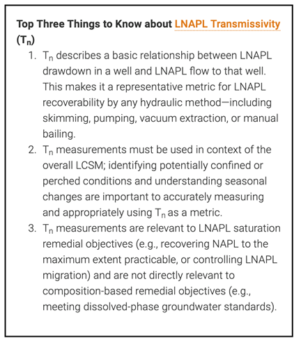
LNAPL Transmissivity : More recently there has a been a move to use LNAPL transmissivity as a key metric to evaluate LNAPL recoverability (e.g., ITRC, 2018). The ITRC’s “Top Three Things To Know about LNAPL Transmissivity” is reproduced to the right.
The use of transmissivity has been catalyzed by a general consensus that hydraulic recovery of LNAPL (skimmer wells, trenches, groundwater pumping, etc.) has a Technology Threshold Metric consisting of LNAPL transmissivity greater than 0.1 to 0.8 ft2/day (0.0093 to 0.074 m2/day). This metric may be used as a decision point for remedial system operation or technology transitions (ITRC, 2018). For example, in the State of Michigan, LNAPL guidance states “if the NAPL has a transmissivity greater than 0.5 ft2/day, it is likely that the NAPL can be recovered in a cost-effective and efficient manner unless a demonstration is made to show otherwise.” (ITRC, 2018). ITRC also describes five sites in detail that were used as the basis of this range (Section 1.3).
LNAPL transmissivity can be determined in two general ways:
- Computer Models: Using a multiphase LNAPL model to calculate transmissivity based on soil type, LNAPL properties, and other factors. The Tier 2 LNAPL Subsurface Volume and Extent Model can be used to easily estimate LNAPL transmissivity, as can LDRM. Sale (2001) provide methods for determining inputs to environmental petroleum hydrocarbon and recovery models.
- Field Measurements (ITRC, 2018, Section 2.0): Conduct field data and analyze the data to calculate the LNAPL transmissivity. ITRC (2018) and ASTM (2013) prescribe three approaches:
- LNAPL Baildown Testing. Note a computer spreadsheet is available to process the data from baildown tests to determine transmissivity (Charbeneau et al., 2012) (no metric units, however).
- Manual LNAPL Skimming Testing.
- LNAPL Recovery System Evaluation.
References
ASTM. 2013. Standard Guide for Estimation of LNAPL Transmissivity. ASTM International.
How can one estimate NSZD?
What is Natural Source Zone Depletion (NSZD)?
NSZD describes the loss of LNAPL due to various processes, the most important of which is biodegradation (ITRC, 2009; ITRC, 2018).
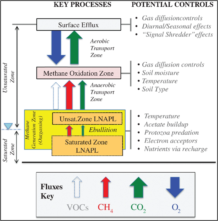
A series of research projects have determined that this depletion is occurring at much faster rates than first thought, up to 100’s to 1000’s of gallons per acre per year (Johnson et al., 2006; Sihota et al., 2011; McCoy et al., 2015; Garg et al., 2017). Additionally, Garg et al. (2017) describes an overview of the latest research and key processes controlling NSZD (see figure to right). As such, NSZD is becoming an important factor in the Conceptual Site Model (CSM) and may be incorporated into site management strategies.
NSZD values reported in the literature range from 2,800 to 72,000 liters per hectare per year with the middle 50% of NSZD values falling between 6,600 to 26,000 liters per hectare per year (Garg et al., 2017).
Additional Resources:
Overview of Natural Source Zone Depletion (NSZD): Processes, Controlling Factors and Composition Change (Garg et al. 2017)
EnviroWiki: Natural Source Zone Depletion (NSZD)
ITRC (2018) Appendix B: Natural Source Zone Depletion (NSZD)
Concawe, 2020. "Detailed Evaluation of Natural Source Zone Depletion at a Paved Former Petrol Station" Concawe Report no. 13/20. https://www.concawe.eu/publication/detailed-evaluation-of-natural-source-zone-depletion-at-a-paved-former-petrol-station/
Lundegard, Paul D., and Paul C. Johnson, 2006. Source Zone Natural Attenuation at Petroleum Hydrocarbon Spill Sites - II: Application to a Former Oil Field. Ground Water Monitoring and Remediation 26 (4): 93–106. https://doi.org/10.1111/j.1745-6592.2006.00115.x.
NSZD Rate Converter
What the Model Does
NSZD rates are typically reported in units of volume of LNAPL biodegraded per area per time, such as “gallons per acre per year” in some of the NSZD projects performed in the United States. This model converts typical measures of NSZD rates between metric and imperial, as well as converting from carbon dioxide flux to mass or volume of LNAPL degraded per area per time (ex. Liters of LNAPL biodegraded per hectare per year).
How the Model Works
The user is able to select an LNAPL type or representative compound, enter an NSZD value and select starting units, and select a final desired unit of mass or volume of LNAPL degradation.
Key Assumptions
For converting from a carbon dioxide flux in units of µmol/m2/sec to an LNAPL volume or mass per area per time, the table below summarizes densities and molecular weights applied for each LNAPL type or representative compound. Note that default parameters apply the density of fresh gasoline (0.77 g/mL), and the molecular weight of octane (114.2 g/mol).
Input Data
Guidance on the selection of specific input parameters for this tool is provided in Section 9.2.1 of the User’s Manual which can be seen here:’
Developer
This LNAPL tool was developed by Poonam Kulkarni of GSI Environmental.
Kulkarni, P., 2021. NSZD Rate Converter, Concawe LNAPL Toolbox.
Inputs:
NSZD Temperature Enhancement Model
What the Model Does
Hydrocarbon degradation can be enhanced with increases in temperature (Sustained Thermally Enhanced LNAPL Attenuation [STELA]) (Zeman et al., 2014; Kulkarni et al., 2017). This model uses the Arrhenius Law to estimate the potential NSZD rate enhancement with any externally created temperature increase up to 45 °C.
How the Model Works
Arrhenius Law estimates for most biological systems, the temperature coefficient is 2.0 (i.e., rates will double with a 10 °C increase in temperature) (Atlas and Bartha 1986; Riser-Roberts 1992).
Q10 = R2/R1[10/(T2-T1)]
Where
Q10 = temperature coefficient, typically 2.0
R1 = NSZD Rate at temperature T1
R2 = NSZD Rate at temperature T2
T1 = Initial temperature (°C)
T2 = Final temperature (°C)
Key Assumptions
For mesophilic anaerobic digestors, optimum temperature range between 30 and 38 °C (Metcalf and Eddy, 1991; Gerardi, 2003). Maximum temperature approximated to be 40 °C, after which bacterial populations decline.
Input Data
Guidance on the selection of specific input parameters for this tool is provided in Section 9.2.2 of the User’s Manual which can be seen here:
Developer
This LNAPL tool was developed by Poonam Kulkarni of GSI Environmental.
Atlas, R.M. , and R. Bartha. 1986. Microbial Ecology: Fundamentals and Applications. Menlo Park, California : Benjamin- Cummings.
Kulkarni, P., 2021. NSZD Temperature Enhancement Calculator, Concawe LNAPL Toolbox.
Gerardi, M.H. 2003. The Microbiology of Anaerobic Digesters. Hoboken, New Jersey : John Wiley & Sons.
Metcalf and Eddy. 1991. Wastewater Engineering—Treatment, Disposal, and Reuse. 3rd ed. New York: McGraw-Hill Publishing Company.
Kulkarni, P.R., King, D.C., McHugh, T.E., Adamson, D.T., Newell, C.J., 2017. Impact of Temperature on Groundwater Source Attenuation Rates at Hydrocarbon Sites. Groundwater Monitoring & Remediation, 37(3): 82-93.
Riser-Roberts, E. 1992. Bioremediation of Petroleum Contaminated Sites. Boca Raton, Florida : CRC Press Inc.
Zeman, N.R. , M.I. Renno , M.R. Olson , L.P. Wilson , T.C. Sale , and S.K. De Long . 2014. Temperature impacts on anaerobic biotransformation of LNAPL and concurrent shifts in microbial community structure. Biodegradation 25: 569–585.
Information on this page can be downloaded using the button at the bottom of the page.
Natural Source Zone Depletion (NSZD) has emerged as an important new remediation alternative for LNAPL sites. Key references and a description of what they explain about NSZD are provided below:
- The ITRC’s (2018) LNAPL Site Management—LCSM Evolution, Decision Process, and Remedial Technologies guidance is heavily influenced by the developments in measuring and applying NSZD for LNAPL site management, with over 100 specific mentions of NSZD in the document and a detailed NSZD appendix. More importantly, it provides detailed information on three frequently used NSZD assessment methods:
- The gradient method, based on soil gas composition,
- Carbon dioxide flux-based methods, including Carbon Traps and dynamic closed flux chambers (i.e. DCC-LI-COR), and
- The biogenic heat monitoring method (Thermal Monitoring).
- Key vendors for these methods are:
- EnviroFlux (Carbon Traps)
- LI-COR (DCC- LI-COR)
- Thermal NSZD (Thermal Monitoring)
- Garg et al.’s (2017) Overview of Natural Source Zone Depletion: Processes, Controlling Factors, and Composition Change provides a detailed review of how NSZD developed, key NSZD processes, potentially NSZD-controlling factors, and how NSZD affects the composition of LNAPL (see graphic to right). It is based on roughly 100 technical references.
- Kulkarni et al.’s (2020) Application of Four Measurement Techniques to Understand Natural Source Zone Depletion Processes at an LNAPL Site describes an extensive research project where four different NSZD measurement techniques were used at a site and then compared.
- Lari et al.’s (2019) Natural Source Zone Depletion of LNAPL: A Critical Review Supporting Modelling Approaches discusses key NSZD processes required to model NSZD and the capabilities of 36 models to accommodate 21 important phenomena.
- ESTCP’s Environmental Wiki has an entry describing NSZD where the significance of NSZD is discussed along with NSZD stoichiometry, the gaseous expression of NSZD through gas evolution, and measuring temperature to determine NSZD (Palaia, T., J. Fitzgibbons, and P. Kulkarni, 2019).
- CRC CARE’s (2018) Technical Report 44: Technical Measurement Guidance for LNAPL Natural Source Zone Depletion provides practical guidance on the measurement of NSZD rates using various available methods. The document applies to hydrocarbon sites that have a need for theoretical, qualitative, or quantitative understanding of NSZD processes. Its Appendix B contains a checklist for practitioners.
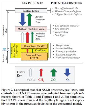
Videos about NSZD
Two videos were developed for the NSZD article in the ESTCP Environmental Wiki. They can be viewed here:
What NSZD Rates are Seen at Hydrocarbon Sites?
The following table from Garg et al. (2017) summarizes measured NSZD rates at various hydrocarbon sites in the U.S. The middle 50% of the NSZD rates range from 700 – 2,800 gallons per acre per year.
What Enhanced NSZD Rates are Feasible?
Hydrocarbon degradation can be enhanced with increase in temperature (Sustained Thermally Enhanced LNAPL Attenuation [STELA]) (Zeman et al., 2014; Kulkarni et al., 2017). Specifically, the Arrhenius Law can be used to estimate the potential NSZD rate enhancement with any externally created temperature increase up to 45°C. The Arrhenius Law estimates for most biological systems, the temperature coefficient is 2.0 (i.e., rates will double with a 10°C increase in temperature) (Atlas and Bartha 1986; Riser-Roberts 1992).
References
Atlas, R.M. , and R. Bartha. 1986. Microbial Ecology: Fundamentals and Applications . Menlo Park, California : Benjamin- Cummings.
Riser-Roberts, E. 1992. Bioremediation of Petroleum Contaminated Sites . Boca Raton, Florida : CRC Press Inc.